Prove Numpy Is Faster Than Normal List (python)

Introduction:

We know numpy is the fast and efficient library to process numeric data that we study in every course of python or data science and on the internet but we don't know how fast numpy really is.

But today I will show you how fast numpy is? and why is that fast over normal python? with an example.

In the next few minutes, you are going to know what is numpy? why is numpy faster than normal python? python array vs numpy array. proof of numpy fastness.

What is numpy:

Numpy open-source python library with the additional support of large, multi-dimensional arrays, matrices, and enrich collections of math operations and array operations.

Using numpy we can achieve c nad c++ like the speed of array processing in python that is not possible without numpy.

Numpy is used to perform wide range of operations on large numerical array in efficient way. and I will prove that in the next section.

Why is numpy faster than python list and how numpy different from python list?

In numpy when we create the numpy array then numpy will allocate contiguous memory block of the array which is different from the python list structure. In python list, it is linked list like structure of small memory blocks each of that can store the only unit amount of data on it.

Numpy array structure is the sequence of memory locations in the disk and python list is collection of the clustered memory locations in the disk.

Memory access in numpy is faster due to the contiguous block of the memory location. Reading and writing of data in memory become easy and fast in numpy arrays. But in the case of numpy list, all memory blocks (segments) are scattered in memory so accessing a particular memory location is hard and slow in python list.

Python list is flexible and numpy array is fast.

Numpy is so fast because it uses a highly optimized library for matrix operations called the BLAS library. This library is written in Fortran and is used in many scientific computing packages. BLAS stands for Basic Linear Algebra Subprograms and is used to perform basic linear algebra operations like matrix multiplication, addition, and subtraction. Additionally, numpy makes use of vectorization and other optimizations that reduce the amount of code needed to perform operations on matrices, drastically reducing the amount of time needed to perform calculations.

proof of numpy fastness:

Example:

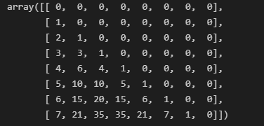
I have created two functions with the same input and same output but different implementations.

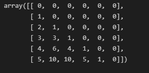
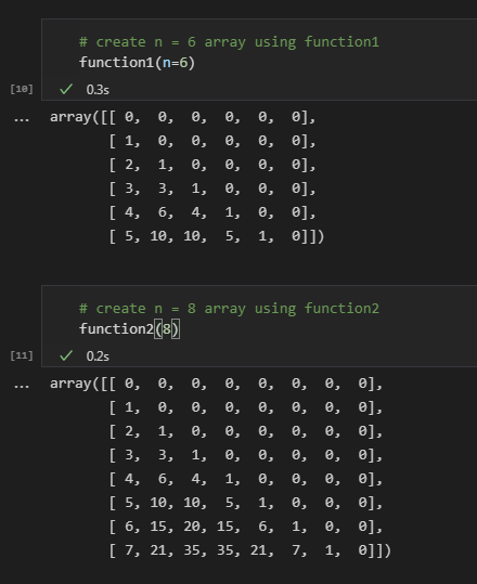
If our input is n = 6 then the output will be:

for n = 8 output will be:

In short, we are creating a pascal triangle inside the two-dimensional array of size n x n.

Both functions take n number as an argument and return a numpy array of size n x n.

Importing needed libraries:

# import numpy and time .
import numpy as np
import time
import matplotlib.pyplot as plt

function1:

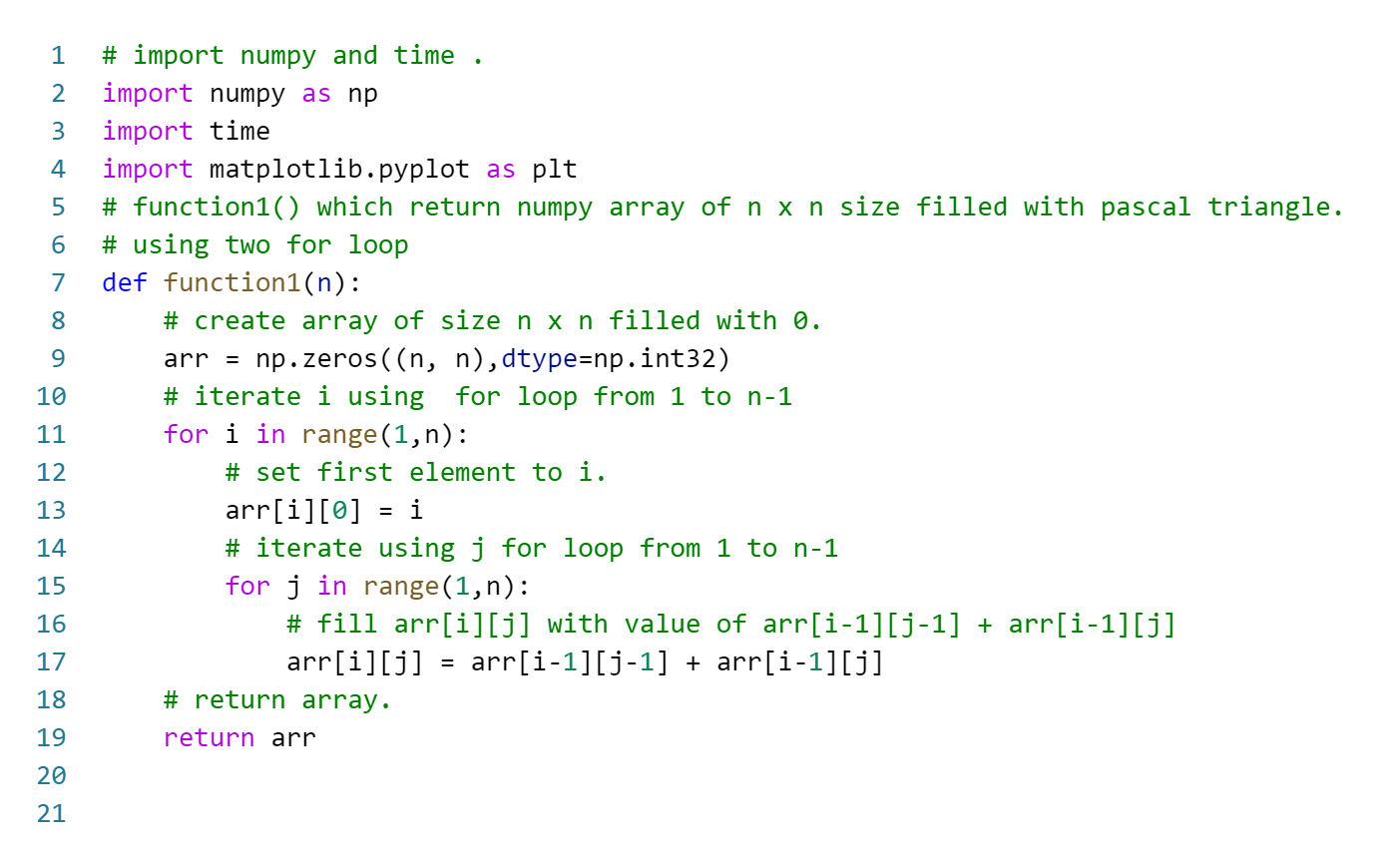
We will be going to implement an addition operation using for loop on created numpy array of size n x n.

function1:

# function1() which return numpy array of n x n size filled with pascal triangle.
# using two for loop
def function1(n):
    # create array of size n x n filled with 0.
    arr = np.zeros((n, n),dtype=np.int32)
    # iterate i using  for loop from 1 to n-1
    for i in range(1,n):
        # set first element to i.
        arr[i][0] = i
        # iterate using j for loop from 1 to n-1
        for j in range(1,n):
            # fill arr[i][j] with value of arr[i-1][j-1] + arr[i-1][j]
            arr[i][j] = arr[i-1][j-1] + arr[i-1][j]
    # return array.
    return arr

function2:

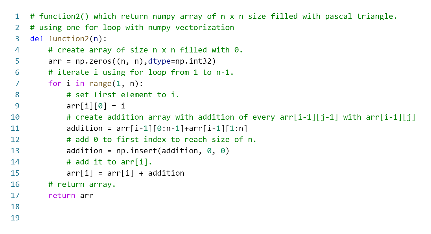
We will be going to implement an addition operation using numpy array addition on created numpy array of size n x n.

function2:

# function2() which return numpy array of n x n size filled with pascal triangle.
# using one for loop with numpy vectorization
def function2(n):
    # create array of size n x n filled with 0.
    arr = np.zeros((n, n),dtype=np.int32)
    # iterate i using for loop from 1 to n-1.
    for i in range(1, n):
        # set first element to i.
        arr[i][0] = i
        # create addition array with addition of every arr[i-1][j-1] with arr[i-1][j]
        addition = arr[i-1][0:n-1]+arr[i-1][1:n]
        # add 0 to first index to reach size of n.
        addition = np.insert(addition, 0, 0)
        # add it to arr[i].
        arr[i] = arr[i] + addition
    # return array.
    return arr

Testing of function1 and function2:

Counting time:

Now, we are going to count time required for specific input not for n = 6 not for n = 8 but for n from [1, 2, 4, 8, 16, 32, 64, 128, 256, 512, 1024, 2048, 4096].

These are numbers that can be generated by simply placing 2's power 0 to 12.

we will count time using the start time and end time as before and after calling functions and with different of them we will find the required time.

For function1:

# list to store execution time.
function1_execution_time = []
# N size.
Ni = 1
for i in range(13):
    # start time.
    start_time = time.time()
    # calling function1()
    function1(Ni)
    # end time.
    end_time = time.time()
    # append difference.
    function1_execution_time.append(end_time - start_time)
    # multiply Ni by 2.
    Ni*=2
    
function1_execution_time

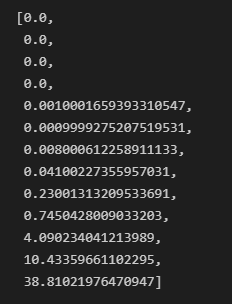
Output for function1:

For function2:

# same as above.
function2_execution_time = []
Ni = 1

for i in range(13):
    start_time = time.time()
    # calling function2()
    function2(Ni)
    end_time = time.time()
    function2_execution_time.append(end_time - start_time)
    Ni*=2

function2_execution_time

Output for function2:

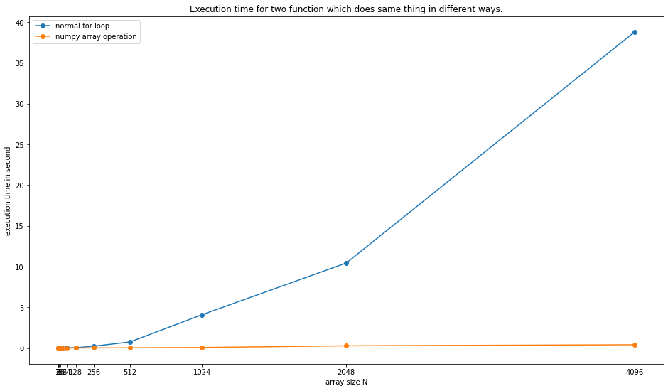
We can see from the above two outputs that function1 time is increasing exponentially with inputs power of 2 as compared to function2.

Plotting:

The latest plot is the graph of the time required for one call vs input power of 2.

# ploting.
plt.figure(figsize=(16,9))
# first line for function1.
plt.plot(x,function1_execution_time,label="normal for loop",marker="o")
# second line for function2.
plt.plot(x,function2_execution_time,label="numpy array operation",marker="o")
# seting label and title
plt.xlabel("array size N")
plt.ylabel("execution time in second")
plt.title("Execution time for two function which does same thing in different ways.")
# set x ticks to x array(size of input.).
plt.xticks(x)
# show legend and plot.
plt.legend()
plt.show()

Output:

graph of the time required for one call vs input power of 2

Conclusion:

With the numpy, we can achieve efficiency and code simplicity in over-program or software. And we can perform large size of array operations efficiently.

Please check this tool created by me to convert the number base from 2 to 20 here: number base converter

Hangman game in cpp and python